A signal teardown of "The World That Bears My Name"
The technical companion to the composition writeup. Same track, opposite lens: what the rendered audio measures, why a beat tracker reads the meter wrong, how the dynamics are engineered across four minutes, and the one master decision the numbers say I got wrong. The why lives in the other post; this is the how.
The composition piece is about what the song means. This one is about what it measures. I pulled the final render back through an analysis pass, partly to write this, partly because I do not fully trust my own ears about my own work and wanted the signal to check my memory. In one place it disagreed with me in a way worth a whole section.
Method and caveats first
The loudness and true-peak figures were measured from the WAV master: 48 kHz, 16-bit PCM, stereo, 246.4 seconds, via ffmpeg's EBU R128 pass. The time- and frequency-domain work (key, meter, structure, spectral profile) ran with librosa on a mono downmix of the 320 kbps distribution render; those measures are robust to lossy encoding and match the master.
There is exactly one place where the MP3 and the WAV disagree, and it is instructive rather than a problem: true peak. I will get to it, because the disagreement is the whole point of measuring from the master.
The spec sheet
| Property | Measured value | How |
|---|---|---|
| Duration | 246.4 s (4:06) | container + sample count |
| Key | B♭ minor | Krumhansl-Schmuckler on CQT chroma, r = 0.69 |
| Tempo (body) | 132.5 BPM | onset-envelope beat tracking, 0:30–3:10 |
| Meter | 3/4 body → 4/4 outro | autocorrelation + session ruler |
| Integrated loudness | -16.7 LUFS | EBU R128, WAV master |
| Loudness range | 15.1 LU | EBU R128, WAV master |
| True peak | -0.01 dBTP | R128 true-peak, WAV master |
| Sample peak | -0.01 dBFS | max abs sample, WAV master |
| Crest factor | ~18.8 dB | sample peak vs integrated RMS |
| Centroid range | 547 Hz → 2544 Hz | per-section spectral centroid |
Key detection is unambiguous; the chromagram shows why
Running a Krumhansl-Schmuckler key estimation against the constant-Q chromagram correlates at 0.69 with the minor profile rooted on B♭, beating every major candidate and every other minor root by a clear margin. The pitch-class energy distribution is the evidence: B♭, C, D♭, E♭ and F dominate, which is exactly the B♭ natural-minor collection, and the chromagram shows that weighting holding steady across the entire track rather than drifting.
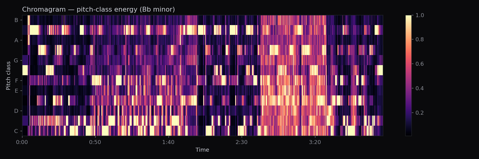
No surprises here, just confirmation. The interesting forensics is one row up.
Meter forensics: why the beat tracker lies
This is the part that earned its own section.
A standard beat-tracking pass returns a clean global tempo of 132 BPM. But when you ask the same algorithm for a frame-by-frame tempo estimate, it wobbles between roughly 115 and 132 BPM with a median near 126. If you only looked at that number you would conclude the track has tempo drift. It does not. It was composed to a hard 132 grid with no tempo automation at all.
The drift is an artifact of the detector trying to fit a 4/4 grid onto a piece that is in 3/4, made worse by the sparse, rubato-feeling solo piano at both ends where there are almost no onsets to lock to. To prove the meter from the signal rather than from the session file, I took the dense body of the track (0:30–3:10, where the percussion is unambiguous) and autocorrelated the onset-strength envelope. The metric grouping with the strongest periodicity above the beat wins.
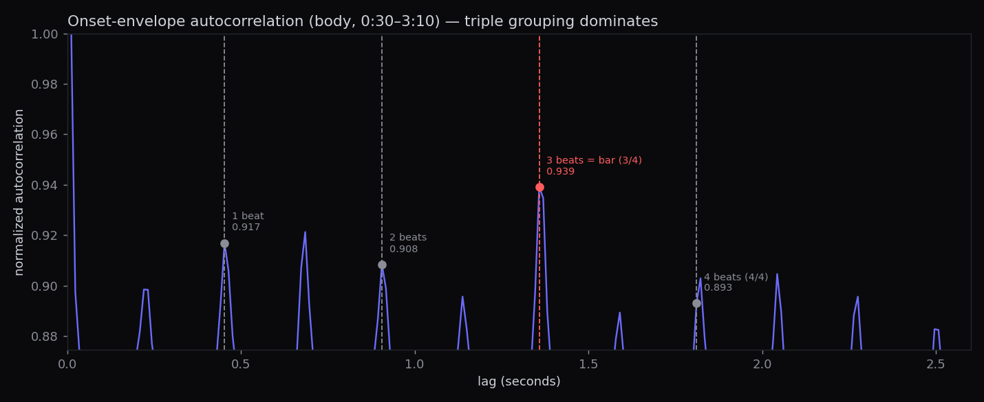
| Grouping | Lag | Normalized autocorrelation |
|---|---|---|
| 1 beat | 0.45 s | 0.917 |
| 2 beats | 0.91 s | 0.908 |
| 3 beats (one bar) | 1.36 s | 0.939 |
| 4 beats | 1.81 s | 0.893 |
The 3-beat lag at 1.36 seconds is the dominant peak. The audio independently confirms triple meter, in agreement with the session ruler. The takeaway for anyone doing automated audio work: a beat tracker's tempo confidence is not meter detection. These algorithms are trained on a corpus that is overwhelmingly 4/4, and they will quietly pattern-match a triple-meter piece into duple subdivisions and report "drift" rather than admit they are in the wrong meter. If you feed music into any system that does automatic beat alignment, tempo-syncs effects, or quantizes to a grid, triple and compound meters are where it will silently misbehave.
The meter change is real and locatable. The session switches to 4/4 at bar 145. At 132 BPM in 3/4, a bar is 1.358 s, so 144 elapsed bars put the switch at ~195.6 s, i.e. 3:16, which lands right where the solo piano outro begins. The piece spends its entire body in three and resolves into four for the final thirty seconds.
Structure and dynamics
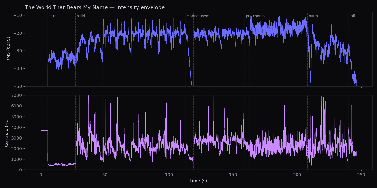
Structural boundaries from an agglomerative segmentation over combined chroma and MFCC features fall at 0:05, 0:27, 0:48, 1:53, 1:59, 2:43, 3:28 and 4:00. Those map cleanly onto the arrangement, and the intensity envelope tells the macro story.
Per-section measurements:
| Section | Time | RMS | Centroid | Sub (20–80 Hz) |
|---|---|---|---|---|
| Intro | 0:05–0:27 | -37 dB | 547 Hz | very low |
| Build | 0:27–1:53 | -22 dB | 2287 Hz | moderate |
| Pre-chorus | 1:53–2:39 | -23 dB | 2544 Hz | moderate |
| Instrumental chorus | 2:39–3:28 | -18 dB | 2132 Hz | highest |
| Solo piano outro | 3:28–4:00 | -28 dB | 2285 Hz | low |
| Tail | 4:00–4:06 | -39 dB | — | gone |
Three things are worth reading off this.
First, the intro sits 19 dB below the chorus. That headroom is reserved deliberately, and it is what makes the dynamic arc possible; you cannot end in a genuine whisper if you never let the start be quiet enough for it to register.
Second, brightness and loudness do not peak together. The loudest section is the instrumental chorus (-18 dB RMS), but the brightest section is the pre-chorus (2544 Hz centroid). The vocal declaration is the moment of maximum spectral clarity; the orchestral catastrophe that follows is louder but darker, because it fills the low end. Onset density confirms the chorus as the rhythmic peak: average onset strength climbs from 0.41 in the intro to 1.04 in the 3:00–3:30 block, then falls off for the outro.
Third, there is a brightness spike to ~6.5 kHz around the 1:00 mark that does not correspond to a loudness peak. That is broadband riser content sweeping upward underneath the second verse, a slow swell that runs nearly the whole build before the arrangement opens up.
Spectral profile and the two engineered low hits
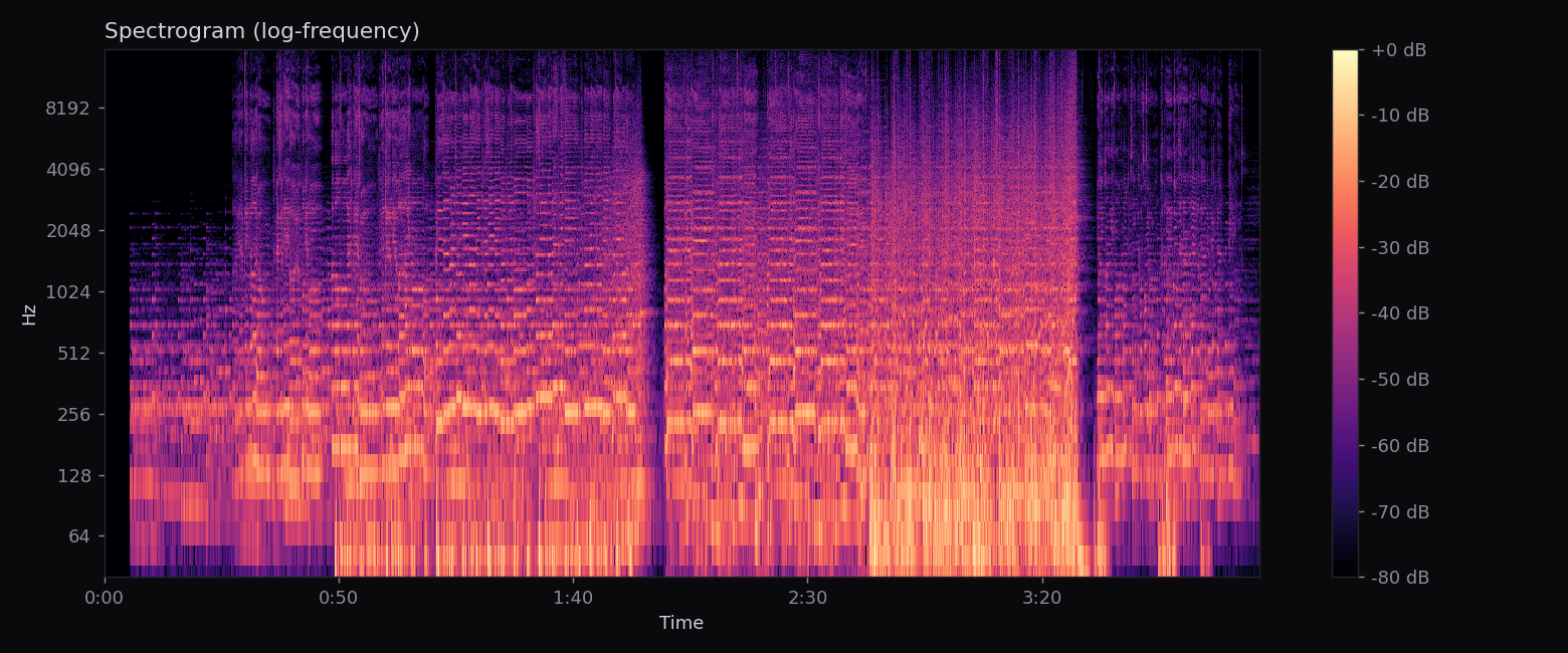
The spectrogram shows the macro shape as a frequency story: a dark, low-banded intro; progressive filling of the upper spectrum through the build and pre-chorus; a dense full-spectrum chorus; and a collapse to a narrow band for the outro piano.
The sub-bass (20–80 Hz) band is almost empty for most of the track and reaches deep in exactly two places, both deliberate. The single strongest sub transient lands at 2:44, the floor of the chorus climax. A second, slightly smaller sub hit lands at 3:32, marking the transition into the solo piano outro like a door closing behind the catastrophe. Those are the only two moments the track commits real energy below 80 Hz, which is why they read as structural punctuation rather than as a continuous bass bed.
Loudness and the master
The track measures -16.7 LUFS integrated with a loudness range of 15.1 LU. That LRA is the headline number of the whole master and the most defensible-yet-arguable decision in it.
Fifteen LU is enormous. A loud modern master typically compresses to somewhere between 4 and 8 LU. Fifteen means the quiet and loud sections are nearly two orders of magnitude apart in perceived level, and that is intentional: the emotional arc from a fragile solo-piano confession to a full orchestral catastrophe cannot survive heavy compression. If the intro is not genuinely quiet, the chorus is not genuinely overwhelming, and the entire dynamic narrative flattens.
This is the main theme of a game, and that context justifies the range in a way a standalone streaming master might not. In-engine, the score sits in a runtime mix with combat SFX, ambience and the game's dynamic audio systems. A master that breathes leaves room for the runtime mix to duck and surface the music dynamically. A brick-walled -9 LUFS master at 5 LU would sit on top of everything and never get out of the way. The crest factor backs this up: roughly 18.8 dB between sample peak and integrated RMS, which is retained transient life rather than a limited slab.
What the numbers say I got wrong
Two issues, smallest first.
True peak is a delivery problem, not a master problem, and measuring both files is what made the distinction visible. The WAV master sits at -0.01 dBTP, under zero, no clipping. But the 320 kbps MP3 I distributed reads +0.03 dBTP, marginally over. The encode introduced inter-sample overshoot that was not in the source, which it can do whenever the master rides the ceiling with no margin, and this master does: sample peak is -0.01 dBFS, essentially peak-normalized to full scale. The master is clean; the file people actually hear is not, by a hair. The fix is a delivery convention rather than a remaster: bounce the WAV at a -1.0 dBTP ceiling before encoding to anything lossy, so the codec has room to overshoot into. The master doesn't clip. The thing I shipped does, and that is a mastering-for-delivery oversight.
The larger issue is a tension I shipped without resolving: the 15 LU range is a gamble against playback reality. It is right for in-engine use and right for the emotional shape, but anywhere the track gets loudness-normalized (streaming, video embeds, storefront trailers), the normalizer pulls integrated level up and the quiet intro ends up higher than intended, eroding the exact fragility the arrangement is built to protect. The correct answer is two masters: the wide-range cut for the game, and a tighter, controlled cut for normalized platforms. I shipped one and hoped. That is the decision I would redo.
Reproducing this
For anyone who wants to run the same teardown on their own renders, the analysis was four passes:
- Loudness:
ffmpeg -i render.wav -af loudnorm=print_format=json -f null -reports integrated LUFS, LRA, true peak and threshold in one shot. - Key:
librosa.feature.chroma_cqtaveraged over time, correlated against the Krumhansl-Schmuckler major and minor profiles at all 12 rotations; highest correlation wins. - Meter:
librosa.onset.onset_strengthover the dense body, thenlibrosa.autocorrelate, then read the normalized peak at 2, 3 and 4 beat-periods. Highest above the beat is your bar grouping. Do this instead of trusting the beat tracker's tempo confidence. - Structure and dynamics:
librosa.segment.agglomerativeover stacked chroma + MFCC for boundaries;librosa.feature.rmsandspectral_centroidper section for the dynamic and spectral profile; a band-limited STFT sum for sub-bass transient location.
Analyze the WAV, not the MP3, if you care about true peak. This track is the textbook case: the WAV reads -0.01 dBTP and the 320 kbps MP3 reads +0.03 dBTP, the encode manufacturing the overshoot. Everything else (loudness, key, meter, structure) survives the lossy round trip unchanged.
That is the song as signal. The version of this track that explains why any of it sounds the way it does is in the composition writeup; this one is just the receipts.